SQL Window Functions Explained: Syntax, Examples & Best Practices 

If you’ve ever written a SQL query that felt longer than it needed to be such as nested subqueries, multiple self-joins, GROUP BY clauses stacked on top of each other; there’s a good chance SQL window functions could’ve reduced that cognitive load in half. Window functions don’t just make queries shorter. They change how you think about data. Once you understand them, you stop seeing rows as independent units and start seeing them as part of a larger, structured picture. That shift is what this blog is about.  

This guide will walk you through everything you need to know about SQL window functions, helping you write cleaner queries, perform advanced data analysis, and solve complex SQL problems with confidence. 

What Are SQL Window Functions? 

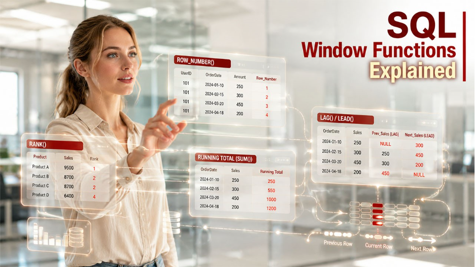
A window function performs a calculation across a specific set of rows called a “window” and returns a value for each individual row in that window. The window itself is defined by an OVER() clause. 

Let’s see what makes them different from regular aggregate functions. When you use SUM() or AVG() with GROUP BY, the query collapses your rows into a single result per group. This makes you lose individual rows. Window functions don’t do that. They calculate across a set of rows and still return a value for every row in the result set. You get both the calculation and the row context. 

That’s the key distinction. It’s also why window functions are so powerful for data analysis. You can compute running totals, rankings, period-over-period comparisons, and moving averages without ever sacrificing row-level detail.   

Understanding SQL Window Function Syntax and Core Components

Before you can use SQL window functions effectively, it’s important to understand the syntax and components that define how calculations are performed across rows.  

The general syntax looks like:  

SELECT column_1, column_2, function() 
OVER (PARTITION BY partition_expression ORDER BY order_expression) 
as output_column_name 
FROM table_name; 

Let’s break down what each part says: 

• SELECT: It defines those columns that you want to pull from the table.  

• function(): It refers to the window function that you’re applying such as ROW, NUMBER(), SUM(), Or LAG().  

• OVER(): This is the core of every window function. It tells SQL to perform the function across a defined window of rows rather than the whole table. 

• PARTITION BY: It divides the result set into partitions based on a column. The window function then runs independently within each partition. If you leave this out, the entire table is treated as one partition. 

• ORDER BY: It determines the order in which rows are processed within each partition. For ranking functions, this is what decides who gets rank 1. 

• output_column_name: It is simply the name you give to the resulting column. 

Note: Window functions run only after SQL has finished processing the WHERE, GROUP BY, and HAVING clauses. This means they always work on the final, cleaned up set of rows; not the raw data. However, if you want to use the result of a window function in a WHERE, GROUP BY, or HAVING clause, you cannot do it directly. You will need a workaround, like wrapping your query inside another query.  

Types of SQL Window Functions You Should Know  

SQL window functions fall into three main categories. Here’s a quick overview: 

Category	Functions	What They Do
Aggregate	SUM(), AVG(), COUNT(), MIN(), MAX(), STDEV(), VAR()	Perform calculations across a window without collapsing rows
Ranking	ROW_NUMBER(), RANK(), DENSE_RANK(), NTILE(), PERCENT_RANK()	Assign a rank or position to each row within a partition
Value	LAG(), LEAD(), FIRST_VALUE(), LAST_VALUE(), NTH_VALUE(), CUME_DIST()	Access values from other rows or return specific positional values

Each category has a distinct job. Aggregate functions handle totals, averages, and counts. Ranking functions sort and number rows. Value functions let you look forward or backward in a dataset which is something regular SQL simply can’t do cleanly.  

Top Benefits of Using SQL Window Functions 

Understanding why SQL window functions are widely used can help you recognize when they’re the right solution for a particular data challenge.  

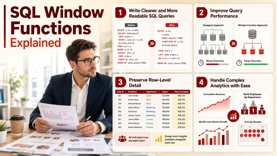
Write Cleaner and More Readable SQL Queries: Window functions eliminate the need for multiple nested subqueries or complicated self-joins. One function often replaces ten lines of messy code. 

Improve Query Performance: Because you’re reducing the number of rows that need to be processed and scanned, queries with window functions often run faster than their subquery-heavy equivalents.   

Preserve Row-Level Detail: Compared to GROUP BY aggregations that return one row per group, window functions keep every original row intact. You get the group-level insight alongside the individual row, which is exactly what most analytical queries need.  

Handle Complex Analytics with Ease: Whether you’re calculating cumulative revenue, ranking employees by department, tracking month-over-month growth, or identifying activity streaks; one consistent syntax handles all of it.  

6 Essential SQL Window Function Patterns for Real-World Analysis 

Only understanding the syntax is not enough. You must know how and when to use these functions for actual problems. That’s where the real skill lies. Here are the six common patterns that come up most often in the real world and in interviews.  

Pattern 1: Find the Latest Row per Group 

This is one of the most common data problems that you’ll face. You have multiple records per user or entity, and you need to find the most recent one. 

The cleanest approach uses ROW_NUMBER() with PARTITION BY on the identifier and ORDER BY on the timestamp in descending order. Each group gets numbered starting from 1, where 1 is the most recent row. Then you filter with WHERE row_num = 1 in an outer query or CTE. 

An alternative is FIRST_VALUE(), which returns the first value in an ordered window. Sort your partition in descending order by date, and FIRST_VALUE() gives you the most recent entry directly. It’s more elegant when you only need a single column, not the entire row.

Pattern 2: Rank Customers, Products, or Events  

Ranking problems are more common than you think. They show up constantly, such as top N products by sales, highest-paid employees per department, or most active users per region. Three functions cover this pattern: ROW_NUMBER(), RANK(), and DENSE_RANK().  

They’re not interchangeable. ROW_NUMBER() always assigns a unique integer to every row, even when values are tied. RANK() assigns the same rank to tied rows but then skips the next number. So, if two rows tie at position 1, the next rank is 3. DENSE_RANK() also gives ties the same rank but doesn’t skip. The next rank after two tied rows at position 1 is 2. 

However, you won’t know when you choose the wrong one. The query runs, it returns results, and nothing tells you that your output is wrong. ROW_NUMBER() is usually the right option for those problems that need exactly one row per position, like “return the top-paid employee per department”.  

Pattern 3: Running Totals and Cumulative Metrics 

Running totals track how a value accumulates over time, like cumulative revenue, total sign-ups to date, or a growing transaction count. The function for this is SUM() used as a window function, with ORDER BY inside OVER(). 

SELECT date, revenue, 
SUM(revenue) OVER (ORDER BY date) AS running_total 
FROM daily_revenue; 

The ORDER BY clause inside OVER() is what activates the cumulative behavior. By default, SQL uses a frame of ROWS BETWEEN UNBOUNDED PRECEDING AND CURRENT ROW. This means that it sums everything from the very first row up to the current one. Add PARTITION BY if you need separate running totals per group, like per customer or per region. 

Understanding database design patterns helps you make smarter decisions about how your data is structured before you start writing window functions on top of it.  

Pattern 4: Compare the Current Row to the Previous or Next Row 

Period-over-period comparisons, time between events, month-over-month growth; all of these need you to reference a row that isn’t the current one. That’s exactly what LAG() and LEAD() are built for. 

LAG() accesses the value from a previous row; N positions back. LEAD() does the same for the following row. Both take the column name, the offset (how many rows back or forward), and an optional default value if the offset row doesn’t exist. 

Before window functions existed, data analysts solved this with self-joins. You’d join a table to itself on a shifted date condition and pray the performance didn’t tank. LAG() and LEAD() replaced all of that with a single, readable function call.  

Pattern 5: Rolling Averages and Time-Window Analysis 

A rolling average doesn’t use all data that is available. It only uses a fixed number of surrounding rows. This makes it useful for smoothing out noise in time-series data and spotting underlying trends in things like daily active users, weekly revenue, or product engagement metrics. 

The function is AVG() with a defined frame clause. For a 7-day rolling average, you’d define the frame as ROWS BETWEEN 6 PRECEDING AND CURRENT ROW, the current day plus the six days before it. As the window moves row by row, the frame stays the same size but shifts with it. That’s the rolling part. 

Depending on what trends you’re trying to surface, you can also use this for 30-day or 3-month rolling windows. The frame clause is what gives you control over the exact scope of each calculation.  

Pattern 6: Retention, Reactivation, and Session Patterns 

This is the most advanced pattern, and it almost always involves chaining multiple windows together. The underlying problem is the classic islands-and-gaps challenge that identifies periods of consecutive activity, known as islands and gaps between them.  

This approach works in layers:  

• First, use LAG() to check whether today’s activity date is exactly one day after yesterday’s. This tells you if a streak is continuing or starting fresh.  

• Then, use SUM() as a window function to calculate a cumulative sum of the “new streak” flags, which generates a unique ID for each streak.  

• Count the rows within each streak ID, and you have your streak lengths.  

• Finally, use DENSE_RANK() to find the top N streaks.  

In this pattern, each CTE has a single and clear job. This layered and logical thinking is what makes this pattern both challenging and impressive, not only in interviews but in real-world analytical work too. Regularly working through problems on coding kata sites is one of the most effective ways to sharpen this kind of layered SQL thinking.  

Common SQL Window Function Mistakes and How to Avoid Them  

It is difficult to recognize these mistakes because they don’t show you errors. Instead, they just return the wrong results.  

Choosing Between ROW_NUMBER(), RANK(), and DENSE_RANK(): If the question asks for the top two employees per job title and two employees are tied for first, RANK() leaves your second position empty. DENSE_RANK() fills it with the wrong person. Only ROW_NUMBER() guarantees exactly one row per position.  

Misunderstanding ORDER BY Inside OVER(): SUM() OVER() without ORDER BY gives you the same grand total in every row. Add ORDER BY and it becomes a running total. Same syntax, completely different output. Easy to miss, painful in an interview. 

Using LAST_VALUE() Incorrectly: When you add ORDER BY inside OVER(), SQL applies a default frame of ROWS BETWEEN UNBOUNDED PRECEDING AND CURRENT ROW. That means LAST_VALUE() actually returns the current row, not the true last row of the partition. Either explicitly set the frame to UNBOUNDED FOLLOWING or just use FIRST_VALUE() with a reversed sort; it’s safer and less error prone. 

Overusing Window Functions Instead of GROUP BY: If you don’t need row-level context, a simple GROUP BY is faster and cleaner. Overusing window functions when they’re not needed is overengineering, and interviewers notice that too.  

Conclusion  

SQL Window Functions are one of those tools that truly transform the way you work with data. They don’t do anything special or out of the world; rather they make complex things simple. Running totals, rankings, trend analysis, and streak detection becomes cleaner, faster, and more readable once you know the patterns.  

The best way to build real fluency is to practice with actual problems. It’s okay even if you get them wrong, understand, and fix them. That’s when you’ll stop recalling syntax and start understanding them.